
HAL Id: hal-01123722
https://hal.science/hal-01123722
Submitted on 5 Mar 2015
HAL is a multi-disciplinary open access
archive for the deposit and dissemination of sci-
entic research documents, whether they are pub-
lished or not. The documents may come from
teaching and research institutions in France or
abroad, or from public or private research centers.
L’archive ouverte pluridisciplinaire HAL, est
destinée au dépôt et à la diusion de documents
scientiques de niveau recherche, publiés ou non,
émanant des établissements d’enseignement et de
recherche français ou étrangers, des laboratoires
publics ou privés.
Left Ventricular Pressure-Volume Analysis : an example
of function assessment on a sheep
Dima Rodriguez
To cite this version:
Dima Rodriguez. Left Ventricular Pressure-Volume Analysis : an example of function assessment on
a sheep. [Research Report] Université Paris Sud. 2015. �hal-01123722�

Research Report
Dima Rodriguez
Left Ventricular
Pressure-Volume Analysis
2010
an example of function assessment on a sheep
Imagerie par Résonance Magnétique Médicale et Mulitmodalité

Left Ventricular Pressure-Volume Analysis:
an example of function assessment on a sheep
Dima Rodriguez
2010
A short version of this work is published in Medical Engineering and Physics Vol. 37, Issue 1, January 2015, pp.100–108
1 Introduction
The evaluation of the left ventricle (LV) performance is of high importance in physiologic investigation
and clinical practice. The diastolic LV function can be assessed by measurements of the ventricular
pressure decline and filling, reflecting relaxation properties, as well as the relationship between pres-
sure and volume during diastole which characterizes stiffness. As for the systolic LV performance,
it is governed by three principal factors, preload, afterload and the contractile or inotropic state of
the myocardium. Preload defines the load on the myocardial fibers just prior to contraction, i.e. the
amount of blood in the ventricle at the end of diastole, while afterload is determined by the external
factors that oppose the shortening of muscle fibers, i.e. arterial impedance. Preload and afterload
determinants can be relatively easily measured or evaluated, but assessing contractile state is far
more difficult. Any index intended to reflect contractility must be load independent.
Common studies evaluate contractility using left ventricular stroke volume (SV), ejection fraction (EF)
and cardiac output (CO). Though intuitive and simple, these parameters are load-dependent and
consequently represent poor contractility indexes. For instance, they are not good indicators of
heart failure and cardiac dysfunction [1, 2].Other studies rely on pressure measurements alone to
assess the LV performance. They evaluate, for example, the maximum rate of pressure change
(dP/dt
max
) which is known to be sensitive to inotropic state and thus correlates with cardiac contrac-
tility. Nonetheless, its load-dependence [3, 4, 5] makes it a weak contractility indicator. The peak
decline of pressure (dP/dt
min
), on the other hand, can quantify isovolumic relaxation, but it cannot
be qualified as an intrinsic relaxation index since it is preload-dependent [6] as well as afterload-
dependent [7]. A widely used parameter for the relaxation quantification is the time constant τ which
characterizes the pressure decay during isovolumic relaxation. Despite being preload-independent
[8], τ cannot be considered an ideal index because of its afterload dependence.
No perfect assessment index can be obtained from volume or pressure alone. Indeed, volume or
pressure measurements on their own are not sufficient to characterize the systolic performance,
they cannot solely define contractility and cardiac response to inotropic agents. Simultaneous pres-
sure and volume measurements are necessary to provide valuable functional parameters. Pressure
indexes can thus be coupled with volume information to negate load dependence. For example,
rather than considering dP/dt
max
, the relationship of this value to end diastolic volume (EDV) can be
2
computed by varying preload conditions. This relationship is linear and its slope provides a preload-
independent contractility index [9]. The relaxation constant τ can also be evaluated over a range of
afterloads and plotted against EDV [10].
In addition, a wide variety of indexes that can be quantified by analyzing pressure-volume (PV) loops
have been proposed to characterize the left ventricle systolic and diastolic performance. For instance
a straightforward characterization of the myocardium stiffness can be obtained from the slope of the
pressure-volume relationship during diastole. Furthermore, a measurement of the ventricular elas-
tance when the contractile forces in the ventricle are at their peak, constitutes a good indicator of the
ventricular contractility and systolic function. Known as end-systolic elastance E
es
, it is independent
of preload, afterload and heart rate [11, 12]. The arterial system, as afterload, can also be assessed
from the PV loop, and, like the ventricle chamber, it can be characterized by its elastance E
a
. Stud-
ies have shown the importance of E
a
as a descriptor of the vascular load and its impact on cardiac
performance [13, 14], indicating that the ratio E
a
/E
es
quantifies the coupling between the ventricle
and arterial system and governs ventriculoarterial matching. Additionally, PV loop area analysis can
provide an evaluation of mechanical energies of a ventricular beat and an assessment of the LV
efficiency.
To measure the ventricle volume, the conductance catheter technique has been used extensively, it
is based on the electrical conductance of the blood contained in the cavity. This technique, nonethe-
less, is based on geometric assumptions, needs volume-dependent calibration and is limited by the
non-linearity of the conductance-volume relation when large volume changes are involved [15]. Fur-
thermore, it relies on Ohm’s law which might not be fully appropriate due to the non-uniformity of
the composition of ventricle and blood, and uses correction parameters that are error prone due to
ventricle geometry and wall thickness changes during contraction [16]. Volume assessment using
cine MRI were proven to yield a more accurate and reliable estimate [16, 17]. For PV loop con-
struction simultaneous volume and pressure measurements are necessary, but given the magnetic
nature of standard pressure sensors, this is problematic during MRI. The pressure signal would be
contaminated by the MR environment and the presence of the sensor would produce artifacts on the
image.
In this report we present a feasibility study for simultaneous pressure measurements using optical
sensors during MRI. In vivo measurements on a sheep are performed and pressure-volume loops
are derived by combining MRI-estimated ventricular volumes with on-site pressure measurements
for various inotropic states. The usual functional indexes are computed, and PV loop analysis is
performed to evaluate the response to inotropic agents.
1.1 Systolic function
The performance of the heart is governed by three principal factors :
1. Preload : the load on the myocardial fibers just prior to contraction, i.e. the amount of blood in
the ventricle at the end of diastole.
2. Afterload : the external factors that oppose the shortening of muscle fibers, i.e. arterial impedance
3. Contractile or inotropic state of the myocardium
The first two determinants can be relatively easily measured or evaluated, but assessing contractile
state is far more difficult. An index of contractility must assess the capacity of the heart to perform
work. Moreover, since changes in loading almost always accompany alterations in the inotropic state
any index intended to reflect contractility must be load independent.
3
1.2 Diastolic function
During diastole the myocardium stops shortening and generating force and relaxes. This results
in a ventricular pressure decline at constant volume (isovolumic relaxation), followed by chamber
filling, which occurs with increasing pressures. The diastolic function is characterized by the my-
ocardium active relaxation properties (calcium recall and sequestration, crossbridge detachment,
ATP metabolism... ) and its passive stiffness (viscoelastic properties of the myocardium ). A de-
crease in ventricular relaxation or increase in ventricular stiffness, reduce the capacities of the ven-
tricular chamber to receive an adequate amount of blood during the diastolic filling phase, and can
lead to diastolic heart failure.
The diastolic function can be evaluated by measurements of the ventricular pressure decline and
filling (onset, rate, and extent) reflecting relaxation properties, as well as the relationship between
pressure and volume during diastole which characterizes stiffness. Although some measurements
mostly reflect the active relaxation and others the passive stiffness, they are closely related (i.e.
processes that affect relaxation also alter stiffness and vice versa).
Even though relaxation is considered a diastolic process, it has a complex interaction with systolic
events. This interdependence can alter the measurement and interpretation of active relaxation. For
instance, the time of onset of active relaxation can alter systolic process but is also affected by the
duration of contraction. It also influences the rate and extent of relaxation which additionally to being
load dependent, would thus be affected by the duration of systole [10].
1.3 Overview of the Pressure-Volume Loop
FillingIC IREjection
LV Volume LV Pressure
Time
ESV
EDV
Aortic valve closes Mitral valve closes
Aortic valve opens Mitral valve opens
Filling
Ejection
Isovulmic Contraction
Isovolumic Relaxation
LV Volume
LV Pressure
ESV EDV
Stroke
Volume
Figure 1 – The Pressure-Volume loop
The PV loop (figure 1) plots the left ventricle pressure versus the ventricle volume. Proceeding anti-
clockwise, the loop traces the chain of events of the cardiac cycle. Systole is represented in the right
and upper boundaries of the loop, while diastole is included in the left and bottom boundaries. At the
4
bottom right corner of the loop is the mitral valve closure point, it occurs at end diastole when the
pressure in the left ventricle exceeds that of the atrium. It is hereby referred to as the end diastolic
point with coordinates (EDV, EDP ). From that point, the isovolumic contraction starts, where the
pressure in the LV increases at a constant volume, until the LV pressure exceeds that of the aorta
causing the aortic valve to open. Once the aortic valve is open ejection starts. The pressure continues
to increase while the chamber volume decreases as the blood is ejected into the aorta, this is known
as rapid ejection. Once the peak systolic pressure is attained, slow ejection starts as pressure and
volume both decrease. This continues until LV pressure becomes smaller than the aortic pressure
causing the aortic valve to close. This point of the cycle is hereby referred to as end-systolic point
with coordinates (ESV, ESP ).The diastolic relaxation now begins. First the ventricle relaxes in an
isovolumic manner, decreasing pressure rapidly at a constant volume, until the opening of the mitral
valve when LVP becomes smaller than the atrium pressure. The blood now flows rapidly into the
ventricle as it completes its relaxation, this is known as the rapid filling phase. The LVP then begins
to increase while the volume increases as blood continues to flow in during the remainder of diastole,
i.e. the slow filling phase (diastasis) and the atrial systole, until the mitral valve closes.
2 Experimental Protocol
The experimental measurements were acquired in collaboration with Emmanuel Durand (Univ. Paris
Sud, CNRS, UMR8081), Ludovic de Rochefort (Univ. Paris Sud, CNRS, UMR8081), Younes Boud-
jemline (Univ Paris 05,Hôpital Necker-Enfants malades, AP HP) , and Elie Mousseaux.(Univ Paris
05,NSERM, U678)
2.1 Animal Preparation
Two female sheep were used in this study. An intervention on the first sheep was performed to com-
pare the optical pressure sensor measurements against the Millar standard probes. A subsequent
intervention on another sheep allowed simultaneous pressure and volume measurements. The ewes
were placed in a sitting position to induce reflex akinesia then anesthetized with a slow injection of
1 g of diluted thiopental. Tracheal tube was inserted and forced ventilation was started with a con-
centration of 1.5-2% isoflurane to maintain anesthesia. To prevent clotting, acetylsalicylic acid (0.5
g) and heparin (3000 IU) were injected intravenously. The carotid artery was catheterized and a vas-
cular dilator was inserted under X-ray monitoring. The animals received humane care in compliance
with the standards of the European Convention on Animal Care. The study was approved by a local
institutional ethics committee (INRA, Paris, France). Qualified personnel supervised the procedures
and adequate anesthesia was used to minimize unnecessary pain.
2.2 In vivo pressure measurements
An optical pressure sensor probe (model OPP-M, Opsens, Quebec, Canada) based on the white-light
polarization interferometry technique was used. The probe tip, 0.4 mm in diameter and 0.5 mm in
length, attached to a 10 m long optical fiber directly transduces pressure into an optical signal which
is then sampled at 1kHz. This device is fully MRI compatible, and immune to radio-frequency effects.
The sensor is linear, with a total error of 2 mmHg and a temperature sensitivity of 0.2 mmHg/°C.
Furthermore, each probe has two specific constant calibration factors.The nude fiber was sheathed
into a non-magnetic 4F catheter (C4F100D, Balt extrusion, Montmorency, France) 1 m in length. The
5
sensor was positioned 5 mm before the catheter tip, facing a slot that had been manually cut in the
catheter wall to ensure pressure transmission. The fiber was then glued into the catheter through
another slot 5 mm above. A null point was set prior to inserting the sensor inside the sheep by
zeroing the measurement at atmospheric pressure.
The validation of the optical probe against a reference pressure transducer (Millar, Houston, USA)
was performed during an aortic intervention that served wider purposes than those stated in the
present report. Guided by X-ray, the OpSens pressure sensor and the Millar catheter were intro-
duced in the sheep’s aorta via the carotid artery. While at the same position in the aortic flow,
pressure signals were recorded simultaneously by both sensors. The animal ventilation was stopped
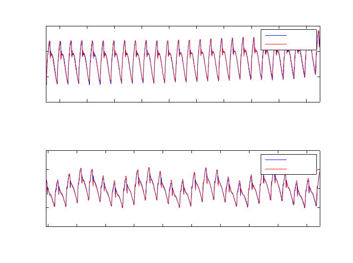
for 20 seconds in order to acquire a stable signal with no respiration modulation. Figure 2 shows
two 20 second extracts of the recorded signals, one while the ventilation was off and another, almost
2 minutes later during normal ventilation. Bland-Altman tests showed that the 95% confidence in-
terval for the limit of agreement is of ±2 mmHg when ventilation was stopped and ±2.2 mmHg with
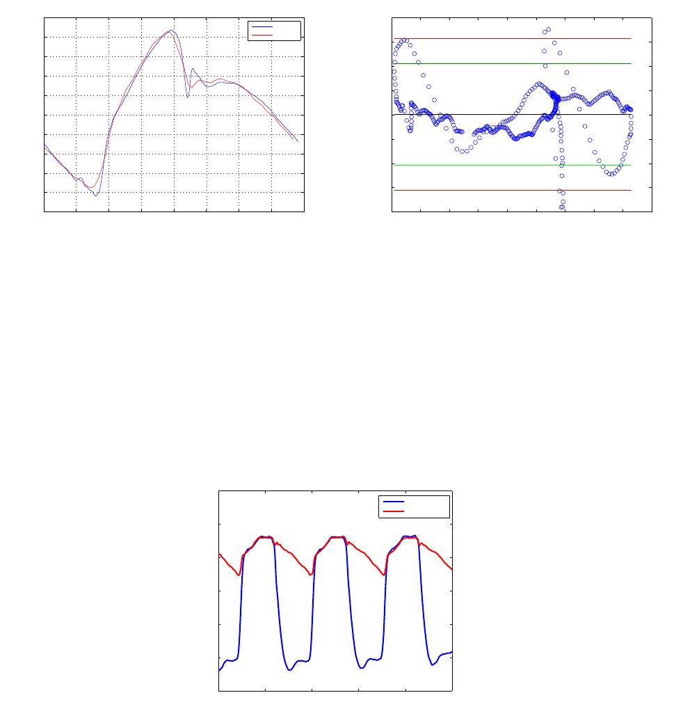
ventilation. The Opsens offset was corrected such that the mean error would be zero. Figure 3a
shows the extracted average cycles of both Opsens and Millar with no ventilation. A Bland-Altman
test (figure 3b) performed on these cycles resulted in a 95% agreement limit of [−1, +1.1]mmHg, and
showed that 99% of measurement differences lie within ±1.6 mmHg. Figure 4 shows an example of
simultaneous measurements of aortic and LV pressure.
18 20 22 24 26 28 30 32 34 36
60
70
80
90
Time (s)
Pressure (mmHg)
No ventilation
Opsens
Millar
138 140 142 144 146 148 150 152 154 156
40
50
60
70
80
Time (s)
Pressure (mmHg)
Ventilation restarted
Opsens
Millar
Figure 2 – Pressure signals recorded using OpSens vs those obtained by the Millar, with and without
ventilation, where the OpSens offset had been corrected.
2.3 Simultaneous in vivo pressure and volume measurements
Pressure measurements with the optical probes were conducted simultaneously with MRI acquisi-
tions in another female sheep (60 kg). After four acquisitions at a baseline condition (heart rate
ranging between 78 and 83 bpm), the sheep was infused dobutamine at a rate of 5 µg/kg/min. Heart
6
0 0.1 0.2 0.3 0.4 0.5 0.6 0.7 0.8
66
68
70
72
74
76
78
80
82
84
86
Time (s)
Pressure (mmHg)
Mean cycle (stopped ventilation)
Opsens
Millar
(a) Opsens and Millar average cycles
68 70 72 74 76 78 80 82 84 86
−2
−1.5
−1
−0.5
0
0.5
1
1.5
2
Average of Opsens and Millar (in mmHg)
Millar − Opsens (in mmHg)
Bland−Altman test for the average cycle
mean − 3 sigma = −1.6
mean + 3 sigma = 1.6
mean − 2 sigma = −1.0
mean + 2 sigma = 1.1
mean = 0.01
(b) Bland-Altman test on the average cycles
Figure 3 – Average cycle comparison
0 0.5 1 1.5 2 2.5
0
20
40
60
80
100
120
Time (s)
Pressure (mmHg)
LV − Aorta
Left Ventricle
Aorte
Figure 4 – Pressures in the LV and the Aorta
7
rate increased to 145-150 bpm and three acquisitions were performed. Dobutamine rate was then
decreased to 2.5 µg/kg/min (heart rate decreased to 125-131 bpm) and a last acquisition was per-
formed before waking the animal up. The whole MR procedure lasted 2 hours and 20 minutes.
2.4 Magnetic resonance imaging acquisitions
Cardiac imaging was performed with a 1.5 T MR scanner (Philips Medical Systems, Achieva) with a
5-element SENSE cardiac array coil and ECG triggering. After calibration and scouting sequences,
true FISP gated cine images (“balanced TFE”) were acquired in 12 sequential 8-mm short-axis slices
(2 mm interslice gap) from the apex to the atrial-ventricular ring, for 30 cardiac phases (TE/TR=
1.7ms/3.4ms, flip angle of 60°, field of view=320 x 240 mm
2
, matrix=256 x 192, voxel size 1.25mm,
echo train length of 10, readout bandwidth 1042 Hz). Mechanical ventilation was continued during the
MRI acquisition procedures without respiratory synchronization. Other sequences were also acquired
for other purposes, not mentioned here.
3 Pressure-Volume loop Computation
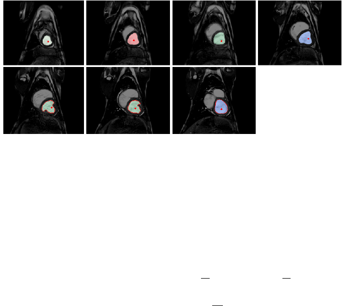
For each slice, the LV was delineated (figure 5) and its area was computed then multiplied by the
slice thickness to derive an elementary volume. These slice volumes were then added up to define
the total LV volume. This was performed for all cardiac phases, and an LV volume evolution in time
was obtained.
Figure 5 – Slices area delineation for a given cardiac phase
During each of the imaging sessions the ventricular pressure was recorded continuously. Since
we only have one volume curve reflecting a somewhat average volume evolution during the image
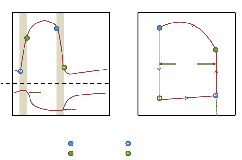
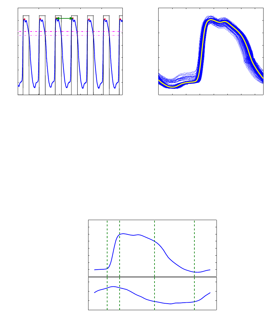
acquisition, an average pressure cycle was derived for the loop computation. Figure 6 summarizes
the cycle calculation. To delimit a heart cycle, pressure peaks were considered to be the end points
of a pressure period. By applying a double threshold on the pressure signal, we delimited individual
windows each containing a pressure peak. Afterward the local maximum is identified inside each
window, thus defining a cycle end point. Once all peaks are determined, individual periods T
i
are
computed, and cycles are extracted between t
peak,i
−
T
i
2
and t
peak,i
+
T
i
2
. These cycles are then
averaged to yield a mean pressure curve. The volume and pressure curves were then associated by
assuming that maximum volume is attained with maximum
dP
dt
. An example of the computed pressure
and volume curves is given in figure 7.
8
65 66 67 68 69 70
0
10
20
30
40
50
60
70
Period extraction
Pressure (mmHg)
Time (s)
T
(a) Extraction of heart cycle
0 0.1 0.2 0.3 0.4 0.5 0.6 0.7
0
10
20
30
40
50
60
70
Time (s)
Pressure (mmHg)
Mean pressure cycle
(b) Averaging over extracted periods
Figure 6 – Mean pressure cycle computation
10
20
30
40
50
60
70
LV Pressure (mmHg)
Pressure and Volume curves
50
70
90
110
Time
LV Volume (ml)
Filling
IC
Ejection
IR
Filling
Figure 7 – Associated LV pressure and volume curves
9
4 Pressure-Volume Analysis
4.1 Stroke volume (SV), Ejection Fraction (EF) and Cardiac Output (CO)
The most straightforward indicators of the pump function of the heart are the stroke volume, ejection
fraction and cardiac output. The stroke volume defines the amount of blood ejected in one heart
cycle. It is computed as SV = EDV − ESV . The ratio of the stroke volume to the total blood volume
present in the ventricle at end systole (EDV ) yields the ejection fraction EF = SV /EDV . The
cardiac output defines the quantity of blood pumped by the heart per time unit and is expressed as
CO = SV ∗ HR, where HR stands for the heart rate. Though intuitive and simple, these parameters
are not sufficient for the evaluation of the cardiac function. For instance, they can’t be relied on for
detecting heart failure and cardiac dysfunction [1, 2]. Moreover, given that they depend on load (EDV,
arterial elastance, ...), they cannot solely characterize contractility and cardiac response to inotropic
agents.
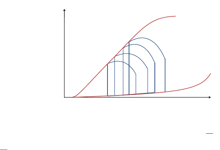
4.2 End-Diastolic Pressure-Volume Relationship (EDPVR)
During the diastolic filling phase, the myocardium behaves as a passive elastic body that is being
stretched, and thus in order to resist deformation, it develops a growing tension as its length increases
with incoming blood. The pressure volume relationship, during this phase, known as the EDPVR, is
generally exponential and depends on the elastic properties of the myocardium, the wall thickness
and the ventricle’s equilibrium volume V
0
[18]. V
0
being defined as the intercept of the EDPVR with
the volume axis, it’s the volume that the ventricle exhibits when subjected to no transmural pressure
(see figure 8).
Volume
Pressure
ESPVR
EDPVR
V
0
Figure 8 – ESPVR and EDPVR
At any given instant of the EDPVR, the ventricle’s stiffness modulus E =
∂P
∂V
is given by the slope
of the tangent to the curve at that point. We can also reason in terms of compliance and compute
C =
∂V
∂P
as the slope reciprocal. Given the exponential nature of the EDPVR, the ratio of pressure to
volume increases as the ventricle continues to fill, thus leading to a decreasing compliance. For small
volumes the ventricle is very compliant, but as the chamber extends it becomes more and more stiff,
as for most biological tissues. The overall chamber stiffness is defined by the myocardium stiffness
as well as the ventricle mass and its mass to volume ratio [10].
10

It’s important to note that the myocardium is not a purely elastic material but also presents viscous
behavior, meaning that the developed pressure, not only depends on the volume extension, but also
on the extension rate (i.e. the filling rate). This dependence implies that for faster filling rates, the
pressures are more elevated for a given volume, and the EDPVR would become steeper. During
diastasis, given that the filling rate is very slow, viscous forces can be ignored, nevertheless they
do contribute to the myocardial response during rapid filling and atrial systole when rates are high.
The viscoelastic effects are however more prominent in atrial systole, than rapid filling when they are
overshadowed by relaxation effects [19].
The EDPVR is independent of the contractility state. When the inotropic state is enhanced (or de-
creased), the diastolic filling portion of the PV loop would remain on this curve while sliding towards
the left (or the right) [20, 21]. This of course leads to compliance alterations in response to inotropic
changes. For instance, decreased contractility would lead to higher ESV, causing a filling at a steeper
portion of the EDPVR, and thus higher stiffness.
In this study the EDPVR is fit with P = α
e
β(V −V
0
)
− 1
, and the compliance is computed using
the slope of the EDPVR during the slow filling phase, thus reflecting purely elastic properties of the
ventricle.
4.3 End-Systolic Pressure-Volume Relationship (ESPVR)
The ESPVR is constructed from a series of PV loops with different ventricular filling volumes. It is
formed by the line connecting the end-systolic points of all PV loops, as shown in figure 8. For a
given contractile state the PV loops are confined beneath the ESPVR curve. This relation can be
approximated as linear in the physiological range and characterized by its slope, the end-systolic
elastance E
es
, which reflects the ventricular contractility state [22, 23] and a volume intercept at a
given pressure that defines its position in the PV plane. Analogous to the force length relationship
of a spring, the ESPVR line can be used for assessing mechanical potential energy and ventricular
efficiency, as will be discussed in a further section.
4.4 End-systolic elastance E
es
Suga et al. [24] viewed the ventricle as having a time varying elastance E(t) =
P (t)
V (t)−V
0
, V
0
being
the intercept of the ESPVR with the volume axis (the theoretic volume for which no pressure is
developed). The slope of the ESPVR gives, thus, a measure of the ventricular elastance when the
contractile forces in the ventricle are at their peak. E
es
is a good indicator of the ventricular contractility
and systolic function, because unlike cardiac output, stroke work and dP/dt, the maximum elastance
is independent of preload after-load and heart rate [11, 12]. Positive inotropic interventions would
increase E
es
and shift the ESPVR to the left, while depressors of the cardiac function would decrease
E
es
shifting ESPVR to the right, nevertheless the volume axis intercept V
0
would not significantly
change [25, 20]. Even though repeated E
es
and V
0
measurements in the intact cardiovascular system
show statistically significant variability because of the autonomic nervous system reflexes, they are
still considered valid indexes of the inotropic state [25].
ESPVR and E
es
estimation The ESPVR is usually obtained by computing several PV loops while
gradually decreasing preload, using a balloon occlusion of the vena cava, for example. This proce-
dure’s invasive nature, limiting clinical applications, has motivated several authors to propose meth-
ods for computing the ESPVR from a single PV loop. Takeuchi et al. [26] simulated end-systolic
11
isovolumic pressure by cosine fitting of the pressure curve, to locate a theoretical P
iso
that would
be attained if ejection did not take place. The E
es
is then computed as the slope of the line con-
necting the point defined by (EDV, P
max
) to the end-systolic point on the PV loop. Other authors
relied on a time-varying elastance model. Senzaki et al. [27] calculated the volume axis intercept
of the elastance curve then defined the ESPVR by connecting this point with the end-systolic point
of loop. Shishido et al. [28] refuted some assumptions made by Senzaki et al. and focused on the
shape of the curve and performed a bi-linear fitting to derive E
es
. Chen et al. [29] later proposed a
simplification of this model.
Although these single-beat estimation methods were tested and validated on humans and other
species, some authors [30] have emitted doubts about their accuracy and their capabilities to as-
sess ventricular contractility. Recently Brinke et al. [11] using Takeuchi’s technique with a modified
fitting scheme (fifth order polynomial instead of a cosine), showed that a good estimation of intercept
volumes can be achieved. They argued that even though the single beat estimation might underes-
timate E
es
and does not agree closely with the vena cava occlusion technique estimation, it is still a
reasonable approach given its experimental advantages.
Since the single beat methods use load dependent elements such as dP/dt and EDV , it is more
valid to view them as load dependent approximations of the load-independent elastance [30].
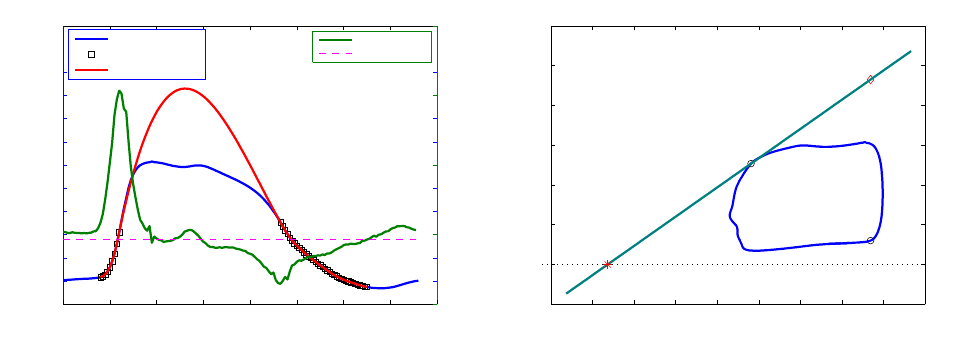
In this study we estimated the ESPVR following the method proposed by Brinke et al. [11]. We
computed a maximum isovolumic pressure P
iso
by using a spline interpolant fitting scheme to fit
the left ventricle pressure curve. We started after end diastole and excluded from the fitting the
pressure data points that lie after dP/dt
max
and before dP/dt
min
and those after the point where
dP/dt increased above 15% of dP/dt
min
. Figure 9 summarizes this procedure.
0 0.1 0.2 0.3 0.4 0.5 0.6 0.7 0.8
0
10
20
30
40
50
60
70
80
90
100
Pressure (mmHg)
Pressure data
considered points
fit curve
0 0.1 0.2 0.3 0.4 0.5 0.6 0.7 0.8
−500
0
500
1000
1500
Time(s)
dP/dt (mmHg/s)
dP/dt
10% dP/dt min
o
Piso
(a) Estimation of P
iso
by fitting the pressure curve
20 30 40 50 60 70 80 90 100 110
−20
0
20
40
60
80
100
120
(EDV,Piso)
(EDV,EDP)
(ESV,ESP)
V
0
ESPVR
Volume (ml)
Pressure (mmHg)
(b) ESPVR in the PV plane
Figure 9 – Single-beat ESPVR estimation
4.5 Time to end systole (T
es
)
Contractility can also be characterized by the duration of systole. Based on the time varying elastance
model, this time can be viewed as the time necessary for E(t) to reach E
es
starting from the onset
of systole (end diastole). T
es
is load independent and shortens with the enhancement of contractility
state [24, 4]. Nonetheless, unlike E
es
, T
es
varies with heart rate [24], thus limiting its use as an
absolute index of inotropy.
12

4.6 Maximal first derivative of pressure (dP/dt
max
)
The maximum rate of change (dP/dt
max
) occurs early during isovolumic contraction, it is sensitive to
inotropic state and thus correlate with cardiac contractility. Nonetheless, its load dependence [3, 4, 5]
makes it a poor contractility index.
To negate preload dependency, rather than considering dP/dt
max
, the relationship of this value to
EDV can be computed by varying preload conditions. This relationship is linear and its slope pro-
vides a preload-independent contractility index which is proportional to the ratio of the E
es
to T
es
[9].
Based on the time varying elastance model, Little [9] gives the dp/dt
max
as
dP
dt
max
= k
E
es
T
es
(V
ED
− V
0
)
where V
0
is the volume intercept of the ESPVR (this means that this relationship and the ESPVR
have the same volume axis intercept) . Since both E
es
and T
es
are load- independent, the slope is
also load independent. Moreover, we know that E
es
increases with enhanced inotropic state, while
T
es
decreases, hence the slope of the dp/dt
max
vs EDV relation would be highly sensitive to inotropic
changes and will increase in response to positive inotropic stimuli [9, 4]. Even though this index is
more sensitive to inotropic changes than E
es
, like T
es
, it depends on heart rate. It was also shown to
be statistically variable at constant inotropic state [31].
As for its afterload dependency, Little [9] argued that it is less sensitive than the ESPVR to alterations
of the arterial characteristics. He showed that the slope of the dP/dt
max
EDV relation remains
somewhat unchanged in response to increase in aortic pressure produced by vasoconstriction, while
the ESPVR is shifted to the left, and its slope is slightly decreased. On the other hand, Mason et al. [5]
discussed that since dP/dt usually peaks at the opening of the semilunar valves, it is deeply affected
by the arterial diastolic pressure. They stipulated that the rate of pressure change is independent
of afterload, only when dP/dt
max
occurs before the onset of ejection (i.e. when diastolic pressure is
very high).
Kass et al. found that in the presence of both preload and afterload alterations, E
es
was relatively
less affected than dP/dt
max
EDV . So, despite E
es
’s lesser sensitivity to inotropic change, its
minimal dependence on both types of load alterations, coupled with its adequate characterization of
contractility, make it somewhat more advantageous than dP/dt
max
vs EDV [4].
4.7 Minimal first derivative of pressure (dP/dt
min
)
The peak decline of pressure (dP/dt
min
) occurs early in diastole, usually shortly after the aortic valve
closure [7] and quantifies isovolumic relaxation. It can’t however be qualified as an intrinsic relaxation
index since it is preload-dependant [6] as well as afterload-dependant [7] (alterations in afterload re-
sult in changes in peak aortic pressure and/or the timing of the aortic valve closure). Moreover, given
the existing interaction between the relaxation process and systolic events, the measure of dP/dt
min
cannot strictly describe the relaxation process, its value could reflect some systolic properties. For
example [6] showed alterations of dP/dt
min
in response to inotropic stimuli.
4.8 Isovolumic relaxation constant (τ)
During isovolumic relaxation, the pressure decay from the time of dP/dt
min
to the time where pres-
sure reaches EDP level, is exponential such that P (t) = P
dP/dt
min
∗ e
−t/τ
and can therefore be char-
acterized by a time constant τ [7] . τ is the time that it takes for the pressure to fall by approximately
two thirds of its initial value. When isovolumic relaxation is slowed, τ is prolonged. Although after-
load dependent, τ was shown to be preload-independent [8]. Usually it is evaluated over a range of
afterloads and plotted against EDV [10].
13
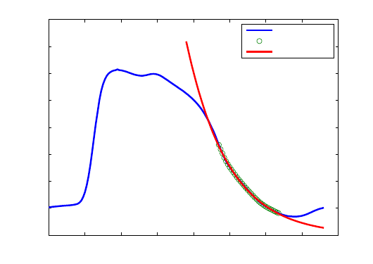
Even if it’s not an ideal index , τ is widely used for relaxation quantification.
In this study, τ is computed using an exponential fit of the pressure points lying between dP/dt
min
and the start of the filling phase (when dP/dt increased above 15% of dP/dt
min
) as shown in figure
10 .
0 0.1 0.2 0.3 0.4 0.5 0.6 0.7 0.8
0
10
20
30
40
50
60
70
80
Time(s)
Pressure (mmHg)
Relaxation time constant estimation
tau = 0.12 s
Pressure cycle
Relaxation
Exponential fit
Figure 10 – Relaxation time constant estimation
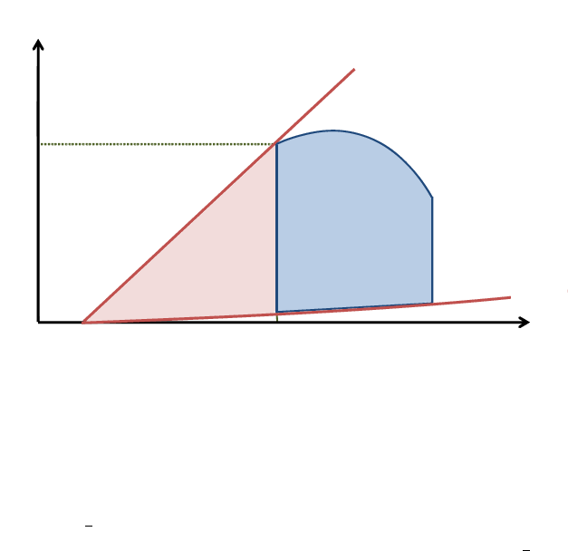
4.9 Effective Arterial Elastance (Ea)
The arterial system, as afterload, can be assessed from the PV loop, and, like the ventricle chamber
it can be characterized by its elastance E
a
. The arterial elastance is determined by the pressure
in the ventricle at end systole, and the amount of blood that the ventricle ejected into the arterial
system. In fact, as the aortic valve closes, the pressure in the aorta is somewhat equal to ESP
and it contains the volume SV , such that its elastance can be computed as E
a
= ESP/SV . It
can be represented on the PV loop diagram as the line connecting the end systolic coordinates and
the EDV point on the volume axis as shown in figure 11. This allows the representation of the
interaction between contractility and afterload in the same diagram, where both are described in
equivalent terms. For instance, for a given contractility state (E
es
) and a given preload (EDV ), when
E
a
increases (stiffer arteries), the SV and EF decrease, and the ESP increases, reflecting the effect
of enhanced afterload.
Indeed this is not a measure of the elastance of the whole arterial tree, and thus is referred to as the
effective arterial elastance. Studies have shown the importance of E
a
as a descriptor of the vascular
load and its impact on cardiac performance [13, 14], indicating that the ratio E
a
/E
es
quantifies the
coupling between the ventricle and arterial system and governs ventriculoarterial matching. This
coupling determines the stroke volume, and defines the ventricle’s energy utilization efficiency to
achieve that SV, as will be discussed subsequently.
4.10 Stroke Work (SW) and Preload Recruitable Stroke Work (PRSW)
The area inside the PV loop has the units of energy (pressure multiplied by volume) and characterizes
the external mechanical work achieved by the heart to eject the SV, this is called the stroke work.
The mechanical energy of contraction produced by the ventricle, i.e. the SW, is stored as hydraulic
14
Volume
Pressure
E
es
V
0
ESV
ESP
EDV
E
a
SV
Figure 11 – Effective arterial elastance
energy in the ejected blood and thus transferred to the arterial system. As in any physical system, the
maximal transfer of energy from the source to the load is achieved when the input impedance of the
load is equal to the output impedance of the source, the source and the load are said to be matched.
Similarly, the energy transfer from one elastic chamber to another is maximal when they both have
the same elastance [32]. Accordingly, maximal SW would occur when E
a
= E
es
.
The SW varies very slightly with afterload but is very sensitive to preload [4] , and thus the study of
the relationship between the EDV and the SW has been judged more suitable. This relationship is
called the preload recruitable stroke work (PRSW). It is a linear relationship [33] which slope reflects
the inotropic state. Slope and elevation increase with positive inotropic stimuli whereas they decrease
in response to negative inotropic agents [20]. It was also shown to be insensitive to afterload over the
physiological range, and thus qualifies as a contractility index, although it might depend on cardiac
geometry and heart rate [33].
Unlike the ESPVR which takes into account end systolic information only, the PRSW integrates data
from the whole cycle. Little et al. [31] showed that the PRSW is less sensitive than the ESPVR to
afterload, its slope is more reproducible (less variable for a given inotropic state) than E
es
, and that
of dP/dt
max
EDV . Its volume intercept is much more stable than that of ESPVR, and dP/dt
max
EDV , and it remains unchanged in response to inotropic stimuli [31]. Nonetheless, the PRSW is less
sensitive to inotropic changes than E
es
and dP/dt
max
EDV [31].
In this study, since preload conditions variation was not performed, the PRSW could not be com-
puted. A method to estimate the slope of PRSW from a single beat was proposed by Mohanraj et al.
[34], however their method did not exclude prior preload variation experiments. For their estimations
they computed an empirical constant from a set of VCO experiments, which they used for the slope
estimation of another group of the same species.
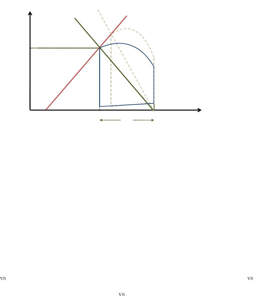
4.11 Potential Energy (PE)
Potential energy, is the mechanical energy that is available in the ventricle at end systole. It is the
energy that was not converted into external work because the aortic valve had closed, and will be
dissipated during relaxation. This energy can potentially produce external mechanical work if there
were no afterload.
15
Volume
Pressure
Slope E
es
EDPVR
V
0
Stroke
Work
Potential
Energy
ESV
ESP
Figure 12 – Mechanical energy
At end systole, the ventricle has a certain pressure ESP for a given volume ESV , it presents a stiff-
ness E
es
, and, like a stretched Hookean spring, stores energy that depends solely on its elongation
and elastance. We know that the potential energy of a Hookean spring that was stretched from its rest
length L
0
to L
s
, is given by
1
2
k(L
s
− L
0
)
2
where k is the spring elastance. Similarly, we can say that
the potential energy that the ventricle holds at end systole would be given by
1
2
E
es
(ESV − V
0
)
2
, this
represents the area under the ESPVR spanning from V
0
to ESV . Note that the part of this area that
lies beneath EDPVR represents energy that is not actively supplied, it results from passive stretching
due to the incoming blood, and the PE release during relaxation can never situate the ventricle under
this curve. Thus, this area portion must not be included for the potential energy calculation. Therefore
the PE is represented by the area of the triangle between the point of end systole on the PV loop, V
0
and the ESV intercept on the EDPVR, as shown in figure 12. The PE thus depends on contractility
(E
es
), passive filling behavior, and afterload (E
a
) which defines end systolic pressure and volume.
Any situation that alters any of these elements, will affect the potential energy.
4.12 Pressure Volume Area ( PVA)
The total mechanical energy of a ventricular beat is known as the pressure volume area and is equal
to the sum of potential energy and stroke work, P V A = P E + SW .
PVA characterizes the ventricle’s oxygen consumption.There is a linear correlation between PVA and
oxygen consumption, V
O
2
increases as PVA increases. Furthermore, the slope of this linear relation
is independent of contractility, but shifts up (or down) as contractility increases (or decreases) [12].
PVA also contains information on crossbridge behavior in a beating heart, and combined with E
es
it
can be used to assess the total amount of Ca
2+
released and removed for contraction [12].
4.13 Mechanical efficiency
Like any other system, the mechanical performance of the ventricle is defined by its ability to convert
metabolic energy into external mechanical work. In other words, it is the ratio of SW (the effective
energy output) to the oxygen consumption (total energy consumption). This ratio is a function of
ventricular loading and contractile state.
16

The mechanical efficiency can be decomposed in two stages :
The efficiency of energy transfer from oxygen to total mechanical energy P V A/V
O
2
. For a given
P V A, this ratio increases with depression of contractility and with afterload [35]. Conversely,
when contractility is enhanced, the V
O
2
vs P V A relation is shifted upwards, more oxygen is
consumed for the same P V A, and thus oxygen conversion efficiency is decreased.
The efficiency of energy transfer from the ventricle to the arterial system SW/P V A, called
cardiac work efficiency (CWE). This is the portion of the total generated energy that is actually
converted into external work. SW/P V A is reciprocally related to
E
a
E
es
[35] which determines the
position of the end-systolic coordinate, thus defining the relative contributions of SW and PE to
the PVA. The cardiac work efficiency increases with contractility enhancement, and decreases
with afterload increase [36]. Studies have shown that the CWE is maximal when
E
a
E
es
= 0.5
[37, 38].
Given the opposite effects of inotropy and afterload on both efficiency indexes, their changes could
compensate when the inotropic state or afterload are altered, leading thus to no changes in the total
mechanical efficiency [35].
Optimal working point To fulfill its pumping function, the heart must transfer enough energy to
the arterial system to ensure adequate flow and perfusion pressure while remaining as efficient as
possible. The cardiovascular system, thus matches the ventricular and arterial properties so that
ventriculoarterial coupling would best achieve that function. As mentioned, CWE is optimized when
the arterial elastance is nearly one half the end systolic elastance, while on the other hand, SW
is optimized when both elanstances are equal. It has been shown that the normal heart at rest
operates at neither maximal CWE (E
a
/E
es
= 0.5) nor maximal SW (E
a
= E
es
), but in fact finds an
optimal working point between the two, which is actually closer to maximal efficiency [37, 38]. SW
might however be favored at the expense of CWE in some cases of mild cardiac dysfunction [38].
5 Results
Pressure-volume loops were computed for all measurements covering four contractility states. Overall
we obtained 9 PV loops : 4 for baseline, 1 with Dobutamine 2.5, 3 with Dobutamine 5 and 1 with
Esmolol.
5.1 Pressure offset correction
Even though the dynamics of the pressure measurements performed here were shown to be ac-
curate, the used pressure sensors present an offset that drifts throughout the experiment, thus in-
troducing an unknown pressure shift between the measurements. This variable drift can exceed 2
mmHg/hour. In order to be able to compare the obtained loops and the extracted parameters, a cor-
rection is necessary to bring the pressure cycles to a common reference. To eliminate these relative
offsets we relied on theoretical fact that the filling parts of all measured PV loops should lie on the
same EDPVR. Hence, we computed that relation for one of the baseline loops (we chose the fourth)
and then shifted the pressure cycles of the rest of the loops so that they would be supported by the
estimated EDPVR. Of course this does not eliminate the “absolute” pressure offset that is added to
17
the reference pressure measurement, but at least all loops now have that same offset and can be
compared.
An attempt to estimate and correct the absolute offset can be made by considering the EDPVR and
ESPVR intersection point. Theoretically these relationships should have the same zero axis intercept.
Thus, we could assume that the absolute offset would be eliminated by shifting the reference baseline
loop so that EDPVR and ESPVR intersect at zero pressure. Of course the same shift would afterward
be applied to the rest of the loops. This procedure would, however, not guarantee the elimination of
the real offset, in fact it depends greatly on the ESPVR estimation, which itself is not very accurate
given that it’s computed from a single beat. Besides given the instability of ESPVR and V
0
and their
variability between repeated measurements [25], the chosen loop probably does not reflect the real
V
0
.
To sum up, the presented pressures here might not actually reflect the real ones, but present a resid-
ual offset that introduces errors in the calculations of some parameters, such as ESP , EDP , P
max
,
V
0
,P E, and E
a
. Other parameters such as E
es
, C , and SW , are independent of the pressure offset
and thus can be assumed accurate even if there’s an unknown shift of the PV loop. Regardless of
whether the offset is important or not, comparison between the considered contractility states re-
mains valid, since the relative offsets are corrected and the absolute shift applies equally to all states.
Further studies will focus on modeling the sensors behavior to enable measurement correction.
5.2 Baseline measurements
Figure 13 shows an example of a baseline loop and some of the extracted parameter values. The
computed mean baseline parameters are compared to values obtained in other studies dealing with
sheep [39, 40, 41, 42, 43, 44] in order to situate our calculations with respect to usual parameter
values. Figure 14 shows a graphical representation of these values for rapid visual comparison.
Some parameters such as E
es
for example agree well with the literature range. Others, like the
compliance and V
0
, differ significantly from what is obtained by other authors. These differences can
be explained by the fact that the sheep studied by those authors are a lot smaller (weighting around 40
kg ) than the one used in our experiments (70 kg). Since the diastolic compliance decreases with the
chamber size [45, 46], smaller animals with smaller hearts have less compliant ventricles. Moreover,
smaller volumes mean that the PV loops are shifted to the left, thus the ESPVR axis intercept is also
shifted to the left, thus explaining the smaller V
0
.
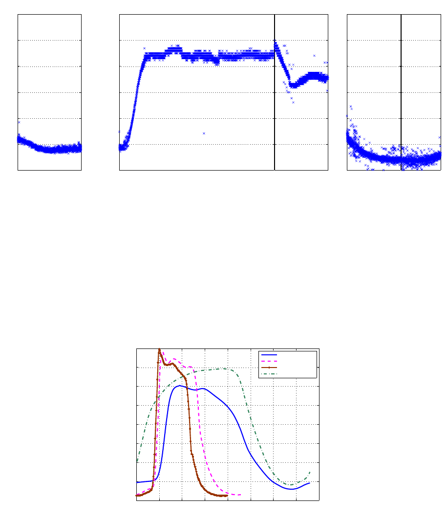
5.3 Contractility states comparison
Figure 15 shows the experimental time line and heart rate evolution throughout the consecutive
states. The instantaneous frequencies were computed, over the pressure recordings, as the inverse
of the time interval separating two pressure peaks, as shown in figure 6a. HRincreases gradually
after the Dobutamine administration starts, it stabilizes then decreases when the Dobutamine rate is
diminished. A HR increase can be observed as we go from one rate to another, as the remaining
Dobutamine might have been injected rapidly to evacuate the tubes for the next perfusion. Esmolol
administration slows down the heart, and as soon as it is stopped, the heart starts recovering. Note
that, the recorded recovery measurements did not last long enough to observe the HR going back to
its normal value.
Of course, functional changes in response to the inotropic agents, go beyond the obvious HR vari-
ation. Not only did the pressure cycle period vary, but its shape was drastically altered. Figure 16
18
20 30 40 50 60 70 80 90 100 110 120
−20
0
20
40
60
80
100
120
Piso = 91.92 mmHg
EDV = 96.89 ml
EDP = 10.97 mmHg
ESV = 68.13 ml
ESP = 49.67 mmHg
V
0
= 34.34 ml
ESPVR
p=1.47 v−50.46
EDPVR
C=5.81 ml/mmHg
SW = 1774.93 mmHg.ml
PE = 592.50 mmHg.ml
Efficiency = 74.97 %
Pressure − Volume loop Analysis
Volume (ml)
Pressure (mmHg)
Figure 13 – Baseline parameter extraction example
Weight HR CWE
20
40
60
80
100
120
140
EDV ESP ESV Pmax V0
−50
0
50
100
150
SV EF EDP
0
10
20
30
40
50
60
70
C CO Ees
0
1
2
3
4
5
6
7
Tes Tau
0
0.1
0.2
0.3
0.4
SW dP/dtmax dP/dtmin PVA PE
−2000
−1000
0
1000
2000
3000
4000
Our Results
Charan 1998
Lee 2010
Bauer 2002
Ratcliffe 2000
Pilla 2003
Segers 2001
Figure 14 – Comparison with the literature
Charan et al. [39], Lee et al. [40] , Bauer et al. [41], Ratcliffe et al. [42], Pilla et al. [43], and Segers et al. [44].
19
0 25’
60
80
100
120
140
160
180
Freq (bpm)
Baseline
1h 2h
Dobutamine 5
2h20’
Dobutamine 2.5
2h30’ 2h50’
Esmolol
3h05’
Recovery
Time
Figure 15 – Frequency evolution throughout the experiment
0 0.1 0.2 0.3 0.4 0.5 0.6 0.7 0.8
0
10
20
30
40
50
60
70
80
Time (s)
Pressure (mmHg)
Mean pressure cycles
Baseline
Dobutamine 2.5
Dobutamine 5
Esmolol
Figure 16 – Mean pressure cycles
20

shows mean pressure cycles, each representing an inotropic state. Contrarily to what would be ex-
pected, the amplitude of the pressure cycle during Esmolol, is higher than that of the baseline. This
could be because the steady state under Esmolol was not reached. Esmolol was administered right
after the Dobutamine, and the measurement time under this state was short.
Esmolol Baseline Dobutamine 2.5 Dobutamine 5
HR (bmp) 78.95 78.28 ± 2.79 129.77 150.99 ± 0
EDV (ml) 99.92 95.22 ± 3.82 69.25 62.31 ± 4.60
EDP (mmHg) 19.27 10.88 ± 0.87 8.77 7.68 ± 0.64
ESV (ml) 77.68 68.55 ± 2.49 43.86 41.72 ± 4.54
ESP (mmHg) 66.90 48.04 ± 3.58 66.99 56.40 ± 8.68
SV (ml) 22.24 26.67 ± 1.84 25.39 20.59 ± 1.40
EF (%) 22.26 27.99 ± 1.16 36.66 33.14 ± 2.88
CO (l/min) 1.75 2.11 ± 0.10 3.29 3.10 ± 0.21
P
max
(mmHg) 69.49 59.46 ± 1.53 78.31 77.64 ± 2.52
C (ml/mmHg) 3.90 6.23 ± 0.47 6.88 8.55 ± 3.35
E
es
(mmHg/ml) 1.55 1.62 ± 0.19 3.83 4.21 ± 0.26
V
0
(ml) 34.64 38.49 ± 3.36 26.35 28.26 ± 6.59
T
es
(s) 0.43 0.30 ± 0.03 0.18 0.15 ± 0
dP
dt
max
(mmHg/s) 510.48 1020.64 ± 20.24 3370.92 3556.28 ± 232.13
dP
dt
min
(mmHg/s) -491.60 -347.02 ± 20.26 -1860.39 -2342.00 ± 428.75
τ (s) 0.10 0.11 ± 0.01 0.04 0.03 ± 0
SW (mmHg.ml) 1301.16 1574.27 ± 183.24 1939.42 1548.46 ± 229.35
PE (mmHg.ml) 1188.56 491.89 ± 107.13 457.67 210.26 ± 84.61
PVA (mmHg.ml) 2489.73 2066.15 ± 238.61 2397.10 1758.71 ± 309.27
CWE (%) 52.26 76.26 ± 4.23 80.91 88.38 ± 3.24
E
a
(mmHg/ml) 3.01 1.81 ± 0.18 2.64 2.74 ± 0.37
E
a
/E
es
1.94 1.12 ± 0.11 0.69 0.65 ± 0.10
Table 1 – Computed parameters for all 4 states
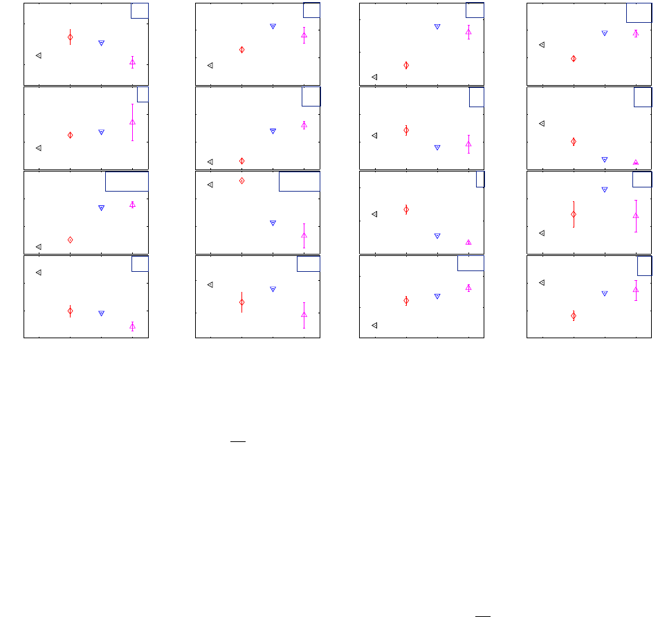
Pressure volume loop analysis was performed for all 9 measurements. The obtained parameter val-
ues are given in table 1. Figure 17 shows a quick visual of the evolution of the computed parameters
as the inotropic state changes.
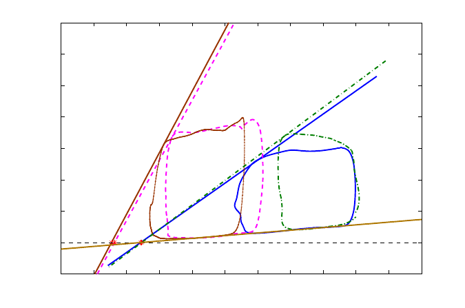
Compared to baseline, E
es
increased significantly with positive inotropic stimuli, but was not consid-
erably changed with Esmolol. As discussed previously, the Esmolol measurement might not be a
good representative of the corresponding state because it was recorded during a transitional state
and does not represent steady state. The ESPVR of the Esmolol loop had even a higher slope than
some of the baseline measurements. Figure 18 shows an example of PV loops representing the four
states (Esmolol, baseline measurement n°4, Dobutamine 2.5, Dobutamine 5 measurement n°2) , as
well their corresponding end-systolic elastances. The time to reach end systolic elastance T
es
did
however show a notable increase between baseline and Esmolol, but this is probably due to its heart
rate dependency.
dP
dt
max
,on the other hand, was more sensitive to inotropic changes, it was reduced
to half its value between baseline and Esmolol. During the period of Esmolol perfusion, the pressure
21
20
30
SV
25
35
EF
2500
3500
CO
60
80
P
max
5
10
C
3
5
E
es
30
50
V
0
0.4
0.5
T
es
2000
4000
dp/dt
max
−2000
−1000
dp/dt
min
0,08
0,16
τ
1400
1800
SW
E B D2.5 D5
500
1000
PE
E B D2.5 D5
1800
2600
PVA
E B D2.5 D5
70
100
CWE
E B D2.5 D5
2
3
E
a
Figure 17 – Analysis parameters for all states
E: Esmolol , B : baseline, D2.5: Dobutamine 2.5 , D5 : Dobutamine 5
dynamics were able to slow down (
dP
dt
max
decreased) but the pressure amplitude remained elevated,
causing an elevated ESP, and thus an elevated E
es
.
As expected, the diastolic compliance increased with inotropic enhancement. As contractility is in-
creased, the PV loops shift to the left on the EDPVR, thus going towards smaller slopes (i.e. stiffness).
The stroke volume measurements confirmed that it is not a good contractility index. In fact, despite the
contractility enhancement, because of its load dependency, the SV of the Dobutamine loop is smaller
than that of baseline. Since the preload (EDV) decreased, so has the SV. The same can be argued
for the EF which did not reflect the inotropic increase induced by the Dobutamine augmentation.
The relaxation process was sped up in response to Dobutamine. Both
dP
dt
min
and τ decreased with
positive inotropic stimuli. The expected opposite effect was, however, not observed for Esmolol. Re-
laxation for Esmolol remained faster than that of baseline. Note that the τ estimation for Dobutamine
is error prone, the relaxation was very fast, leaving only a few points on the pressure relaxation curve
for the exponential fitting.
Increasing the Dobutamine concentration did not enhance the stroke work (the SV decreased with
an insignificant increase in maximum pressure), it did however somewhat enhance the cardiac work
efficiency. Conversely, the CWE diminished notably with Esmolol.
The ESPVR axis intercept V
0
varies slightly among states but not distinctly enough to be attributed to
contractility changes. Theoretically V
0
is independent of the inotropic state [24], all ESPVR and ED-
PVR should meet at the same axis intercept. The changes observed here account for the instability
of V
0
[25] as well as measurement and estimation errors. Note that the V
0
range here is affected by
the pressure offset and its correction.
The effective arterial elastance E
a
increases with inotropic enhancement as ESP is increased. The
ventriculoarterial coupling index E
a
/E
es
decreases when contractility increases. At baseline, this
index is close to 1, indicating that the ventricle is working near maximal SW. With Dobutamine, E
a
/E
es
22
is approximately 0.6, thus the heart is functioning around the optimal working point between maximal
SW and maximal CWE, while remaining closer to maximal efficiency. During Esmolol perfusion, the
coupling index is close to 2, the functioning mode is far from optimal, and widely inefficient.
10 20 30 40 50 60 70 80 90 100 110 120
−20
0
20
40
60
80
100
120
140
Pressure − Volume loop Analysis
Volume (ml)
Pressure (mmHg)
E
es
=1.47
E
es
=3.83
E
es
=3.91
E
es
=1.55
Dobutamine 2.5
Esmolol
Baseline
Dobutamine 5
EDPVR
Figure 18 – End-systolic elastance for all contractility states
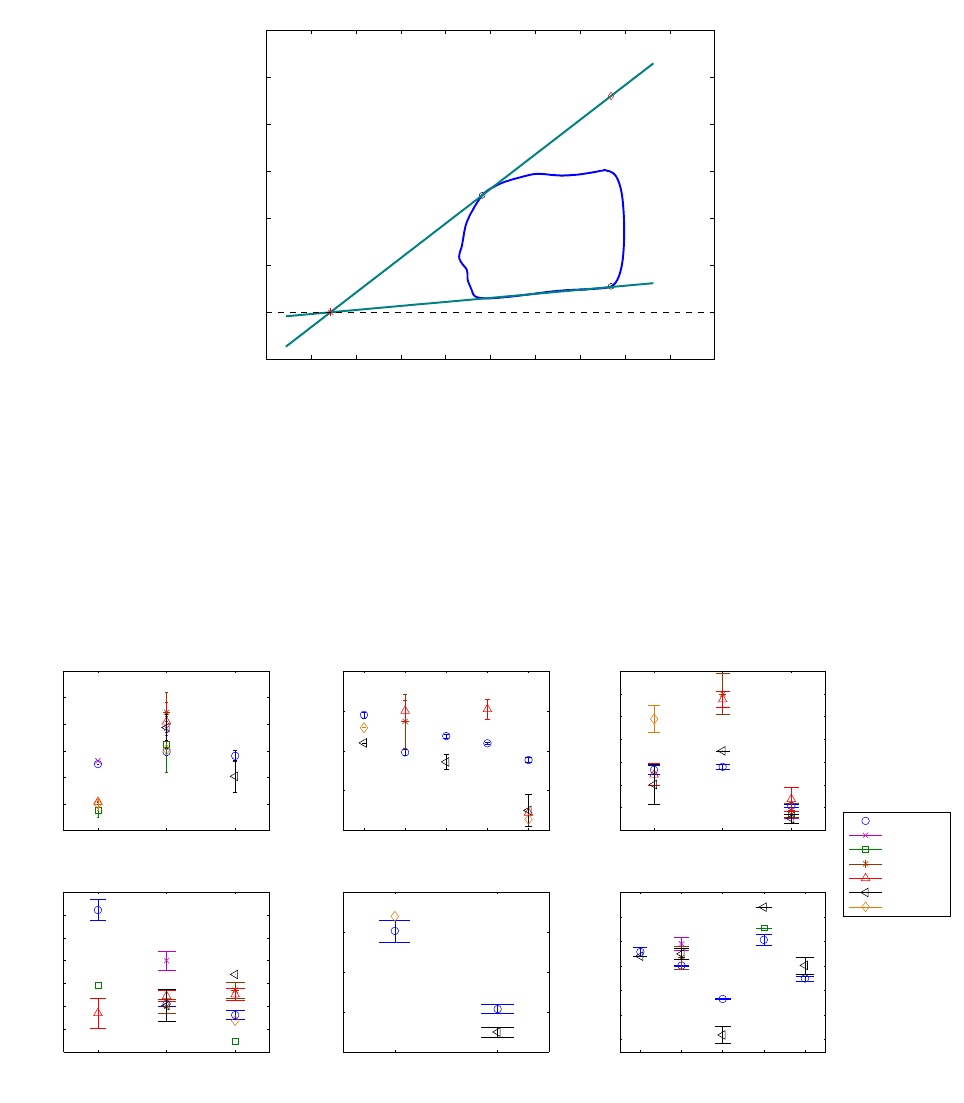
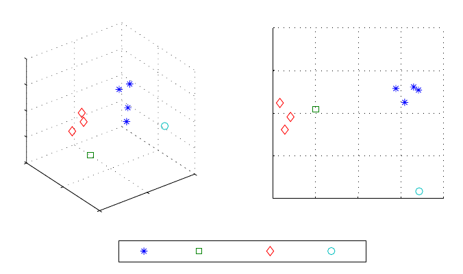
5.4 Principal component states representation
The PV loop analysis is done here by examining a large number of parameters N, some of which
correlate with each other. Each loop is thus characterized by N variables. To represent a loop
measurement, we need an N-dimensional space. However given that correlations exist between the
parameters, the number of dimensions can be reduced using principle component analysis (PCA).
With this method a new coordinate system is formed by new parameters which are derived as linear
combinations of the old ones. A measurement can thus be represented by a reduced number of
variables which are somewhat independent. Our computations have shown that the N parameters
can be reduced to 3 or even 2 with no significant loss. Figure 19 shows the 9 measurements projected
on a 3D and a 2D coordinate system, where the axis are linear combinations of the N parameters.
This allows the visualization of sate clusters where the measurements corresponding to the same
state are grouped.
This PCA procedure can be exploited for measurement classification. Having derived the principle
component from a training set of measurements (such as we have here), given a new measure-
ment we could, with a classification scheme, determine in which state the measurement has been
recorded.
6 Discussion
MRI is considered to be the gold standard for absolute cardiac volume measurements. Obtaining PV
loops requires simultaneously recording pressure during the MRI sessions. Pattynama et al.[47] used
a Millar micromanometer to achieve such measurements, and argued that because it is made from
23
−5
0
5
−5
0
5
−4
−2
0
2
4
3D PCA
B D2.5 D5 E
−4 −2 0 2 4
−4
−2
0
2
4
2D PCA
Figure 19 – 2D and 3D representation by principal component analysis
brass the obtained pressure signals were not significantly altered, however, some image artifacts
were observed. Schmitt et al.[48] and Kuehne et al.[49] used liquid filled catheters to measure ven-
tricular pressure down a 1m pressure line. The impedance of the transmission line reduces pressure
amplitudes, and constitutes a low pass filter that attenuates high frequency components. A pressure
sensor placed inside the ventricle would provide a more accurate representation of the actual LV
pressure. The use of optical sensors in this study enabled pressure measurements directly in the
ventricle without any interaction with the MRI acquisition.
Study limitations
Unlike the conductance catheter technique, PV loop calculation using MRI imposes the use
of an average pressure cycle vs average volume instead of instantaneous pressure vs instan-
taneous volume. Thus, the PV loop here reflects a global performance cycle and does not
take into account an exact punctual correspondence between individual volume and a pressure
measurements.Moreover the time synchronization between the volume and pressure cycle in
this study was done based on bibliographic data, a more accurate match could be achieved by
using the pressure signal to trigger the image acquisition and thus synchronize both waveforms.
Due to the lack of real-time volume recordings, it was impossible to obtain a series of load
varying PV loops using MRI because a steady state over several cycles is needed in order to
compute a volume. For the same reason, the assessment of contractility transit states is not
possible using MRI. This remains, for now, an advantage in favor of the conductance technique,
however, future advances in MRI may enable the overcoming of this limitation.
An attempt to correct the pressure offset was made here but pressure values might not be
representatives of the real values. If we assume that we only have an additive offset term on
pressure, some parameters can still be considered accurate despite the unknown offset, such
as E
es
, C ,SW , τ , .... Other parameters, however, such as V
0
, P E, E
a
necessitate the knowl-
edge of the real offset value. There might also be an amplification term in the pressure sensors,
this would have further effects on the estimated parameters. The pressure sensors need to be
characterized and their behavior must be modeled to correct pressure measurements
24
The computed PV loop indexes depend greatly on the measurement accuracy, whether MR
volume estimations, or pressure sensor accuracy. We don’t really have an assessment of either.
A more comprehensive study including several animals must be carried out to confirm the
results and conclusions given here.
List of abbreviations
CO Cardiac Output
CWE Cardiac Work Efficiency
EDP End Diastolic Pressure
EDPVR End-Diastolic Pressure-Volume Relationship
EDV End Diastolic Volume
EF Ejection Fraction
ESP End Systolic Pressure
ESPVR End-Systolic Pressure-Volume Relationship
ESV End-Systolic Volume
HR Heart Rate
IC Isovolumic Contraction
IR Isovolumic Relaxation
LV Left Ventricle
LVP Left Ventricle Pressure
MR Magnetic Resonance
MRI Magnetic Resonance Imaging
PE Potential Energy
PRSW Preload Recruitable Stroke Work
PV Pressure-Volume
PVA Pressure Volume Area
SV Stroke Volume
SW Stroke Work
VCO Vena Cava Occlusion
25
References
[1] M. Maeder and D. Kaye. Heart failure with normal left ventricular ejection fraction. J. Am. Coll.
Cardiol., 53(11):905 – 918, 2009.
[2] K. Gaddam and S. Oparil. Diastolic dysfunction and heart failure with preserved ejection fraction:
rationale for raas antagonist/ccb combination therapy. Am J Hypertens, 3(1):52 – 68, 2009.
[3] W. Grossman, F. Haynes, J. Paraskos, S. Saltz, J. Dalen, and L. Dexter. Alterations in preload
and myocardial mechanics in the dog and in man. Circ. Res., 31:83–94, 1972.
[4] D. Kass, W. Maughan, Z. Guo, A. Kono, K. Sunagawa, and K. Sagawa. Comparative influence of
load versus inotropic states on indexes of ventricular contractility: experimental and theoretical
analysis based on pressure-volume. Circulation, 76:1422–1436, 1987.
[5] D. Mason, E. Braunwald, J. Covell, E. Sonnenblick, and J. Ross. Assessment of cardiac contrac-
tility: The relation between the rate of pressure rise and ventricular pressure during isovolumic
systole. Circulation, 44:47–58, 1971.
[6] P. Cohn, A. Liedtke, J. Serur, and E. Sonnenblick. Maximal rate of pressure fall (peak negative
dp/dt) during ventricular relaxation. Cardiovasc. Res., 6:263–267, 1972.
[7] J. Weiss, J. Frederisken, and M. Weisfeldt. Hemodynamic determinants of the time-course of
fall in canine left ventricular pressure. J. Clin. Invest., 58:751–760, 1976.
[8] S. Varma, R. Owen, M. Smucker, and M. Feldman. Is tau a preload-independent measure of
isovolumetric relaxation? Circulation, 80:1757–1765, 1989.
[9] W. Little. The left ventricular dp/dt max -end-diastolic volume relation in closed-chest dogs. Circ.
Res., 56:808–815, 1985.
[10] M. Zile and D. Brutsaert. New concepts in diastolic dysfunction and diastolic heart failure: Part
I:diagnosis, prognosis, and measurements of diastolic function. Circulation, 105:1387–1393,
2002.
[11] E. Brinke, R. Klauts, H. Verwey, E. van der Wall, R. Dion, and P. Steendijk. Single-beat estimation
of the left ventricular end-systolic pressure-volume relationship in patients with heart failure. Acta
Physiol., 198:37–46, 2010.
[12] H Suga. Global cardiac function: mechano-energetico-informatics. J. Biomech, 36(5):713–720,
May 2003.
[13] K. Hayashida, K. Sunagawa, M. Noma, M. Sugimachi, H. Ando, and M. Nakamura. Mechanical
matching of the left ventricle with the arterial system in exercising dogs. Circ. Res., 71:481–489,
1992.
[14] R. Kelly, C. Ting, T. Yang, C. Liu, W. Maughan, M. Chang, and D. Kass. Effective arterial
elastance as index of arterial vascular load in humans. Circulation, 86:513–521, 1992.
[15] M. Danton, G. Greil, J. Byrne, M. Hsin, L. Cohn, and S. Maier. Right ventricular volume mea-
surement by conductance catheter. Am. J. Physiol.-Heart C., 285:1774–1785, 2003.
[16] C Jacoby, A Molojavyi, U Flogel, MW Merx, ZP Ding, and J Schrader. Direct comparison of
magnetic resonance imaging and conductance microcatheter in the evaluation of left ventricular
function in mice. Basic Res. Cardiol., 101(1):87–95, JAN 2006.
26
[17] E. M. Winter, R. W. Grauss, D. E. Atsma, B. Hogers, R. E. Poelmann, R. J. van der Geest,
C. Tschope, M. J. Schalij, A. C. Gittenberger-de Groot, and P. Steendijk. Left ventricular func-
tion in the post-infarct failing mouse heart by magnetic resonance imaging and conductance
catheter: a comparative analysis. Acta Physiol., 194(2):111–122, OCT 2008.
[18] S. Glantz and R. Kernoff. Muscle stiffness determined from canine left ventricular pressure-
volume curves. Circ. Res., 37:787–794, 1975.
[19] J. Gilbert and Glantz S. Determinants of left ventricular filling and of the diastolic pressure-
volume relation. Circ. Res., 64:827–852, 1989.
[20] M. Dickstein, O. Yano, H. Spotnitz, and D. Burkhoff. Assessment of right ventricular contractile
state with the conductance catheter technique in the pig. Cardiovasc. Res., 29:820–826, 1995.
[21] J. Thomas and A. Weyman. Echocardiographic doppler evaluation of left ventricular diastolic
function. physics and physiology. Circulation, 84:977–990, 1991.
[22] W. Grossman, E. Braunwald, T. Mann, L. Mclaurin, and L. Green. Contractile state of the left
ventricle in man as evaluated from end-systolic pressure-volume relations. Circulation, 56:845–
852, 1977.
[23] H. Mehmel, B. Stockins, K. Ruffmann, K. von Olshausen, G. Schuler, and W. Kubler. The linearity
of the end-systolic pressure-volume relationship in man and its sensitivity for assessment of left
ventricular function. Circulation, 63:1216–1222, 1981.
[24] H. Suga, K. Sagawa, and A. Shoukas. Load independence of the instantaneous pressure-
volume ratio of the canine left ventricle and effects of epinephrine and heart rate on the ratio.
Circ. Res., 32:314–322, 1973.
[25] J. Spratt, G. Tyson, D. Glower, J. Davis, L. Muhlbaier, C. Olsen, and J. Rankin. The end-systolic
pressure-volume relationship in conscious dogs. Circulation, 75:1295–1309, 1987.
[26] M. Takeuchi, Y. Igarashi, S. Tomimoto, M. Odake, T. Hayashi, T. Tsukamoto, K. Hata, H. Takaoka,
and H. Fukuzaki. Single-beat estimation of the slope of the end-systolic pressure-volume relation
in the human left ventricle. Circulation, 83:202–212, 1991.
[27] H. Senzaki, C. Chen, and D. Kass. Single-beat estimation of end-systolic pressure-volume
relation in humans. Circulation, 94:2497–2506, 1996.
[28] T. Shishido, K. Hayashi, K. Shigemi, T. Sato, M. Sugimachi, and K. Sunagawa. Single-beat
estimation of end-systolic elastance using bilinearly approximated time-varying elastance curve.
Circulation, 102:1983–2989, 2000.
[29] C. Chen, B. Fetics, E. Nevo, C. Rochitte, K. Chiou, P. Ding, M. Kawagachi, and D. Kass. Nonun-
vaasive single-beat determination of left ventricular end-systolic elastance in humans. J. Am.
Coll. Cardiol., 38:2028–2034, 2001.
[30] K. Kjorstad, C. Korvald, and T. Myrmel. Pressure-volume-based single-beat estimations cannot
predict left ventricular contractility in vivo. Am. J. Physiol.-Hear t C., 282:1739–1750, 2001.
[31] W. Little, C.P. Cheng, M. Mumma, Y. Igarashi, J. Vinten-Johansen, and W. Johnston. Compar-
ison of measures of left ventricular contractile performance derived from presure-volume loops
in conscious dogs. Circulation, 80:1378–1387, 1989.
27
[32] K. Sunagawa, W. Maughan, and K. Sagawa. Optimal arterial resistance for the maximal stroke
work studied in isolated canine left ventricle. Circ. Res., 56:586–595, 1985.
[33] D. Glower, J. Spratt, N. Snow, J. Kabas, J. Davis, C. Olsen, G. Tyson, Sabiston D., and J. Rankin.
Linearity of the frank-starling relationship in the intact heart : the concept of preload recruitable
stroke work. Circulation, 71:994–1009, 1985.
[34] K. Mohanraj and M. Feneley. Single-beat determination of preload recruitable stroke work rela-
tionship:derivation and evaluation in conscious dogs. J Am Coll Cardiol., 35:502–513, 2000.
[35] T. Kameyama, H. Asanoi, S. Ishizaka, K. Yamanishi, M. Fujita, and S. Sasayama. Energy con-
version efficiency in human left ventricle. Circulation, 85:988–996, 1992.
[36] T. Nozawa, Y. Yasumura, S. Futaki, N. Tanaka, M. Uenishi, and H Suga. Efficiency of energy
transfer from pressure-volume area to external mechanical work increases with contractile state
and decreases with afterload in the left ventricle of the anesthetized closed-chest dog. Circula-
tion, 77:1116–1124, 1988.
[37] M. Starling. Left ventricular-arterial coupling relations in the normal human heart. Am. Heart J.,
125:1659–1666, 1993.
[38] H. Asanoi, S. Sasayama, and T. Kameyama. Ventriculoarterial coupling in normal and failing
heart in humans. Circ. Res., 65:483–493, 1989.
[39] NB Charan, R Ripley, and P Carvalho. Effect of increased coronary venous pressure on left
ventricular function in sheep. Resp. Physiol., 112(2):227–235, MAY 1998.
[40] Lawrence S. Lee, Ravi K. Ghanta, Suyog A. Mokashi, Otavio Coelho-Filho, Raymond Y. Kwong,
R. Morton Bolman, III, and Frederick Y. Chen. Ventricular restraint therapy for heart failure: The
right ventricle is different from the left ventricle. J. Thorac. Cardiovasc. Surg., 139(4):1012–1018,
APR 2010. 35th Annual Meeting of the Western-Thoracic-Surgical-Association, Banff, CANADA,
JUN 24-27, 2009.
[41] F Bauer, M Jones, T Shiota, MS Firstenberg, JX Qin, H Tsujino, YJ Kim, M Sitges, LA Cardon,
AD Zetts, and JD Thomas. Left ventricular outflow tract mean systolic acceleration as a surro-
gate for the slope of the left ventricular end-systolic pressure-volume relationship. J. Am. Coll.
Cardiol., 40(7):1320–1327, OCT 2 2002.
[42] MB Ratcliffe, AW Wallace, A Salahieh, J Hong, S Ruch, and TS Hall. Ventricular volume, cham-
ber stiffness, and function after anteroapical aneurysm plication in the sheep. J. Thorac. Car-
diovasc. Surg., 119(1):115–124, JAN 2000.
[43] JJ Pilla, AS Blom, DJ Brockman, VA Ferrari, D Yuan, and MA Acker. Passive ventricular con-
straint to improve left ventricular function and mechanics in an ovine model of heart failure sec-
ondary to acute myocardial infarction. J. Thorac. Cardiovasc. Surg., 126(5):1467–1476, NOV
2003.
[44] P Segers, P Steendijk, N Stergiopulos, and N Westerhof. Predicting systolic and diastolic aortic
blood pressure and stroke volume in the intact sheep. J. Biomech., 34(1):41–50, JAN 2001.
[45] G. Diamond, J. Forrester, J. Hargis, W. Parmley, R. Danzig, and Swan J. Diastolic pressure-
volume relationship in the canine left ventricle. Circ. Res., 29:267–275, 1971.
[46] J. Forrester, G. Diamond, W. Parmley, and Swan J. Early increase in left ventricular complinace
after myocardial infarction. J. Clin. Invest., 51:598–603, 1972.
28
[47] P. Pattynama, A Deroos, E Vandervelde, H Lamb, P Steendijk, J Hermans, and J Baan.
Magnetic-Resonance-Imaging Analysis Of Left-ventricular Pressure-Volume Relations - Valida-
tion With The Conductance Method At Rest And During Dobutamine Stress. Magn. Reson.
Med., 34(5):728–737, NOV 1995.
[48] B. Schmitt, P. Steendijk, K. Lunze, S. Ovroutski, J. Falkenberg, P. Rahmanzadeh, N. Maarouf,
P. Ewert, F. Berger, and T. Kuehne. Integrated assessment of diastolic and systolic ventricular
function using diagnostic cardiac magnetic resonance catheterization: Validation in pigs and
application in a clinical pilot study. J. Am. Coll. Cardiol. Img., 2:1271–1281, 2009.
[49] T. Kuehne, S. Yilmaz, P. Steendijk, P Moore, M. Groenink, M. Saaed, O. Weber, C. Higgins,
P. Ewret, E. Fleck, I. Nagel, E. Schulze-Neick, and P. Lange. Magnetic resonance imaging
analysis of right ventricular pressure-volume loops: In vivo validation and clinical application in
patients with pulmonary hypertension. Circulation, 110:2010–2016, 2004.
29
